DL2 Gradient descent

• Youtube: Gradient descent, how neural networks learn | Deep Learning Chapter 2

Key Takeaway

• Learning = minimizing the cost function by nudging every weight and bias in the direction that reduces cost
• That direction is given by the negative gradient
• Backpropagation is how we compute that gradient efficiently

This chapter answers:
How does a neural network actually learn?

Introduce

Learning in neural networks = adjusting weights and biases to make predictions less wrong.

• This chapter: how the network updates parameters.
• Core idea: Gradient Descent.

Two Main Goals of This Video

• Understand the intuition of gradient descent.
• Connect that intuition to neural network parameters (all weights and biases).

What Should Learning Optimize?

We need one number that says “how bad the network currently is”.

• This number is called the cost (or loss over dataset).
  • If cost is high, predictions are bad.
  • If cost is low, predictions are better.

Cost Function (Simple Form)

A cost function is a mathematical formula used to measure how wrong a model’s predictions are.

Neural Network function:

• Input: 784 pixels
• Output: 10 numbers (0~9)
• Parameters: 13,002 (weights/bias)

Cost function is:

• Input: 13,002 (weights/bias)
• Output: 1 number (the cost)
• Parameters: many, many, many training examples

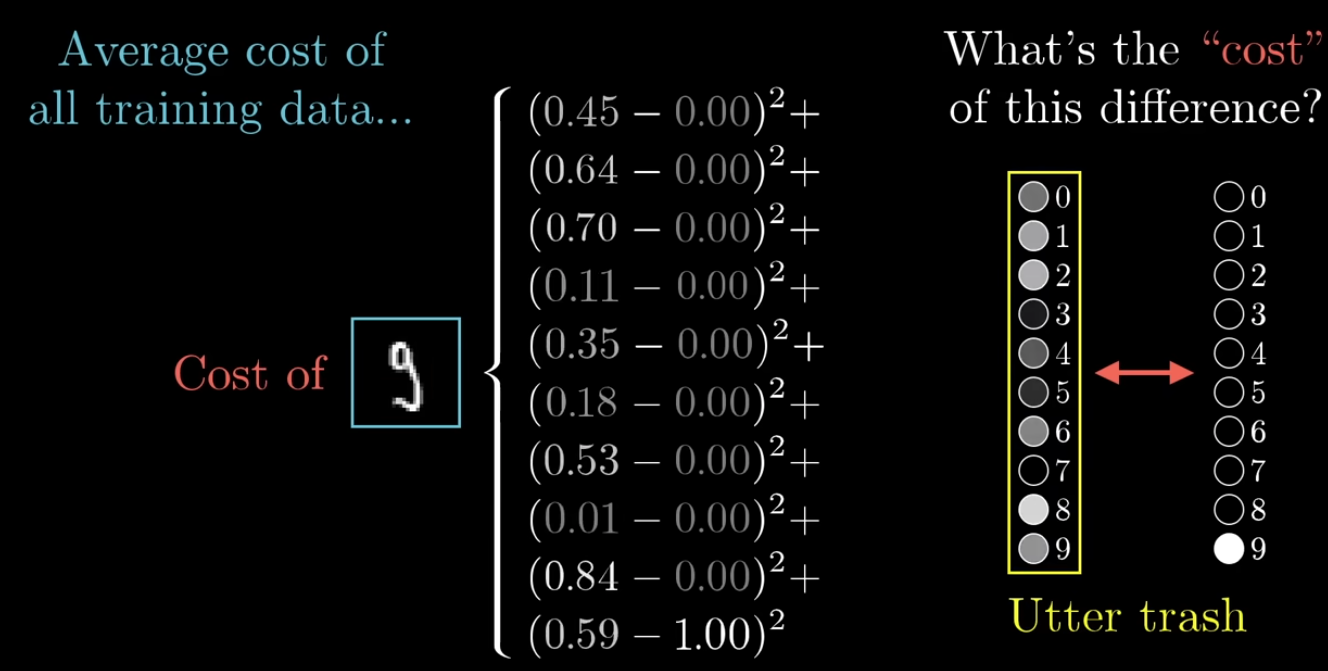
For one training example:

$$L=\sum _j(a_j-y_j{)}^2$$

• $a_j$: output activation of neuron $j$
• $y_j$: target value of neuron $j$
• Squaring has two main purposes:
  • It prevents positive and negative errors from canceling each other out
  • It penalizes larger errors more heavily

Cost Function = Average loss over all training examples
$C(w,b)=\frac{1}{N}{\sum }_{x\in \text{training set}}L(x;w,b)$

• average: $\frac{1}{N}$
• sum all training set: ${\sum }_{x\in \text{training set}}L(x)$
• $C$ is the average error over the training set.
• Learning goal: make $C$ as small as possible.

Find the min cost point of cost function

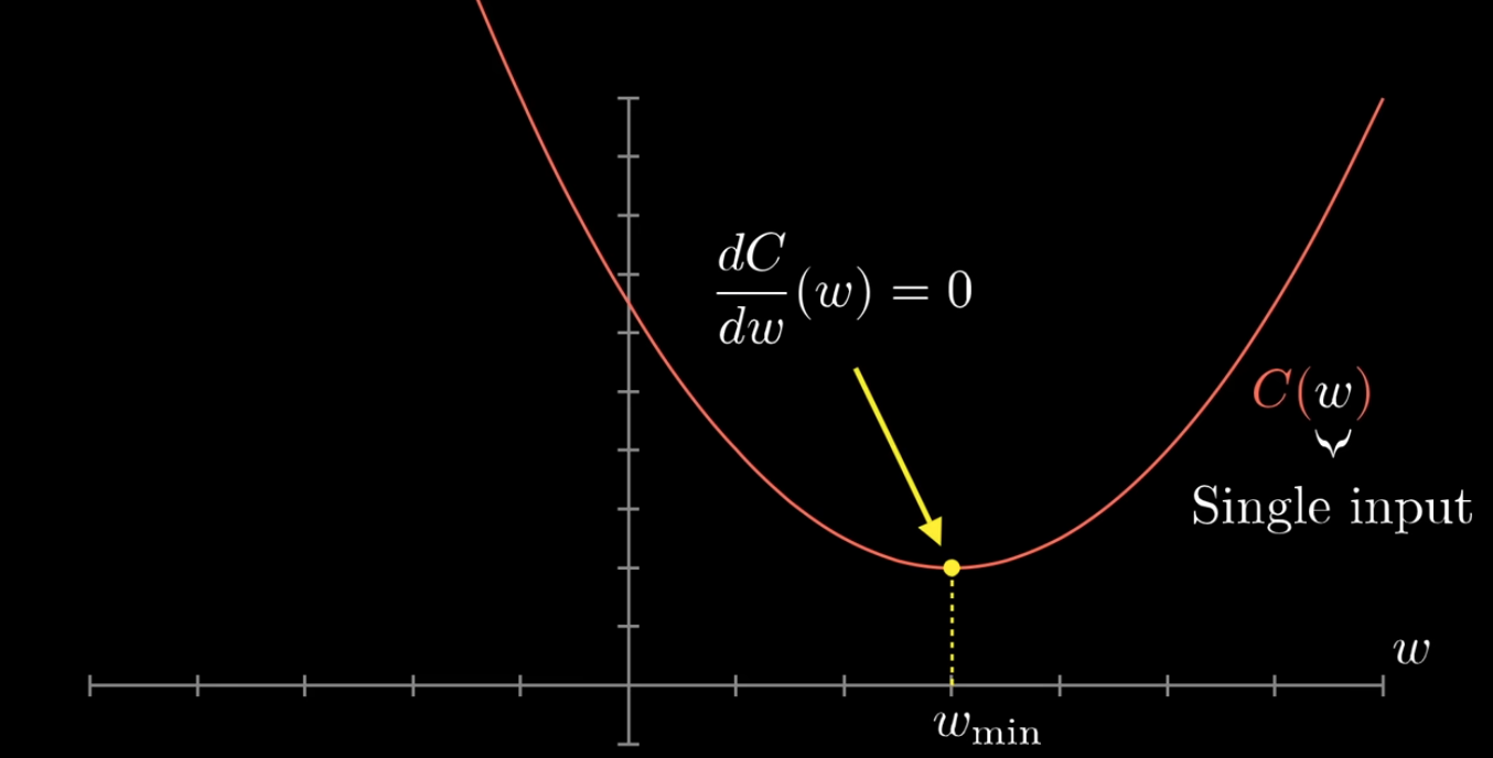
• Cost Function Curve for a Single Weight

Explain derivative

• Derivative = the instantaneous rate of change of a function.

• Cost function as C(w) because different values of w produce different cost values;

  • compute the derivative $\frac{dC}{dw}$​ to see whether the cost is increasing or decreasing at the current w
  • and use that slope information to adjust w step by step until C(w) gets closer to its minimum.

• The figure labels: $\frac{dC}{dw}(w)=0$

  • This means: $\frac{dC}{dw}$ is the derivative of C(w) with respect to w
  • the derivative tells us the slope of the curve
  • at the minimum point, the curve is flat

• so the slope is zero, $\frac{dC}{dw}=0$ at the bottom of the curve.

Gradient Descent

Imagine the cost function as a landscape (hills and valleys). We want to move downhill.

Gradient descent (∇ = gradient symbol):

• is the method the model uses to learn.
• It works by repeatedly adjusting the parameters (weights and biases) a little bit so that the cost function becomes smaller.
• At each step, it looks at the gradient, which tells how the cost changes with respect to each parameter, and then moves the parameters in the opposite direction of that gradient.
  • Parameters (all weights + biases) are coordinates in a high-dimensional space.
  • At current position, compute the slope direction that increases cost fastest.
  • Move in the opposite direction to decrease cost fastest.

Update Rule

If parameter vector is $\theta$:
$\theta \leftarrow \theta -\eta \nabla C(\theta )$

New parameters = old parameters - a small step opposite to the gradient.

• Symbols mean:
  • θ: parameter
  • $C(\theta )$: cost function
  • $\nabla C(\theta )$: gradient vector (all partial derivatives)
  • $\eta$: learning rate (step size)
• the model adjusts its parameters a little bit each step in order to reduce the cost.

For each parameter separately:

$$w_i\leftarrow w_i-\eta \frac{\partial C}{\partial w_i},b_i\leftarrow b_i-\eta \frac{\partial C}{\partial b_i}$$

new value = old value - learning rate × the partial derivative of the cost with respect to that parameter

Why Gradient?

• Gradient points to steepest increase of the function.
• Negative gradient points to steepest decrease.
• So using $-\nabla C$ is the most efficient local direction to reduce cost.

Learning Rate (η)

Links: What is Gradient Descent - GeeksforGeeks

• Learning rate is a important hyperparameter in gradient descent
• that controls how big or small the steps should be when going downwards in gradient for updating models parameters.
• It is essential to determines how quickly or slowly the algorithm converges toward minimum of cost function.
  • If Learning Rate too small:
    • Learning is very slow.
  • If Learning Rate too large:
    • May overshoot and bounce around, or even diverge.
• Practical training needs a reasonable learning rate schedule.

High-Dimensional Perspective

• A small network can already have thousands of parameters.
• Real networks can have millions or billions.
• We cannot visualize this space directly, but gradient descent still applies mathematically.

Why Random Initialization?

• If all weights start the same, many neurons stay symmetric and learn the same thing.
• Random initialization breaks symmetry.
• Then different neurons can learn different useful features.

---

Example

Example 1: One-Parameter Gradient Descent

• Suppose: $C(w)=(w-3{)}^2$

• Then: $\frac{dC}{dw}=2\ast (w-3)$

• Let initial $w_0=0$, learning rate $\eta =0.1$.

  • Step 1:
    • Gradient at $w=0$
      • $slope=2\ast (0-3)=-6$
    • Update: $w_1=w_0-\eta \cdot slope=0-0.1(-6)=0.6$
  • Step 2:
    • Gradient at $w=0.6$
      • $slope=2\ast (0.6-3)=-4.8$
    • Update: $w_2=w_1-\eta \cdot slope=0.6-0.1(-4.8)=1.08$

• You can see $w$ gradually moves toward 3, where cost is minimal.

• Update formula stays the same no matter whether the slope is negative or positive;

  • only the direction of the update changes. $w_{new}=w_{old}-\eta \cdot slope$
  • if $slope=\frac{\partial C}{\partial w_i}=0$, so w does not change, and it may mean we have already reached the minimum point.

Example 2: Network Parameter Update (Conceptual)

• Suppose one weight has derivative $\frac{\partial C}{\partial w}=0.25$.
  • If $\eta =0.01$:
  • $w_{new}=w_{old}-0.01\times 0.25=w_{old}-0.0025$
• If the derivative is positive, increasing $w$ increases the cost, so we move $w$ smaller.
• If the derivative is negative, increasing $w$ decreases the cost, so we move $w$ larger.

---

Summary

• Neural network learning is an optimization problem.
• Define cost, compute gradients, update parameters repeatedly.
• Gradient descent is the core engine behind this process.
• Chapter 2 builds the optimization intuition; Chapter 3 explains backprop in detail.

---

Derivative Power rule

$\frac{d}{dx}(x^n)=n{x}^{n-1}$Examples:

• $\frac{d}{dx}(x^2)=2x$
• $\frac{d}{dx}(x^3)=3x^2$
• $\frac{d}{dx}(x^4)=4x^3$