DL3 Backpropagation (intuitively)

• Youtube: Backpropagation, intuitively | Deep Learning Chapter 3

Key Takeaway

• Backpropagation passes error backward from the output layer
• Each weight’s desired change is proportional to: how wrong the output was × how active the sending neuron was × how many neurons send similar signals
• The final gradient is the average of these nudges over all training examples

This chapter answers:

How do we compute which weight/bias should change, and by how much?

Introduce

Backpropagation is the core algorithm that tells every parameter how it should move to reduce cost.

• Key intuition: start from output error, pass responsibility backward layer by layer.

Recap

• Network forward pass:
  • Input image $x$ (784 pixels) goes through layers.
  • Output layer gives activations $a^L$ (10 numbers for digits 0~9).
• Training target:
  • Minimize cost $C(\theta ;D)$
    • θ = model parameters (weights, biases)
    • D = dataset (training data)
  • Find the best set of parameters θ so that the model’s error on the dataset DDD is as small as possible.
• Gradient descent update: $\theta \leftarrow \theta -\eta \nabla C(\theta )$
• Missing piece before this chapter:
  • How to compute all partial derivatives efficiently.

---

What’s cost of the different?

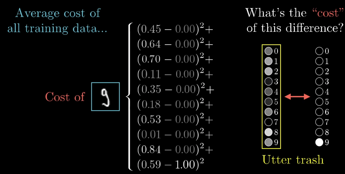
• know the total cost of the network
  • $L={\sum }_j(a_j-y_j{)}^2$

• $-\nabla C(\text{all weights and biases})=\left[\begin{array}{c}0.17\\ 0.80\\ -0.87\\ ⋮\\ -0.04\\ 1.58\\ 1.59\end{array}\right]$

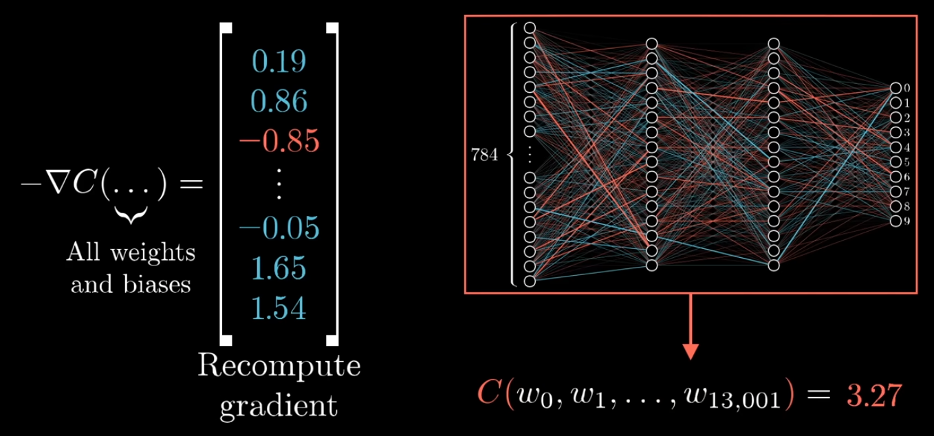
• The gradient vector is built component by component. Each component is a partial derivative with respect to one parameter, computed while keeping all other parameters fixed.

• See details: Cost vs Gradient in Neural Networks

---

Neural network contains many parameters (weights and biases). During training, these parameters are adjusted using gradients to minimize the cost function.

To lower the cost effectively, we need to know how each parameter affects the final output. However, computing the gradient for every parameter one by one would be far too inefficient.

That is why we use backpropagation. It is an efficient algorithm for computing the gradients of all parameters in the network.

Backpropagation

Backpropagation uses the chain rule to pass the final error backward through the network, so we can compute each layer’s gradients efficiently.

Process

Start from the final cost
	↓
Determine how the output layer affects the cost
	↓
Determine how the previous layer affects the output layer
	↓
Determine how earlier layers affect the previous layer
	↓
Propagate backward layer by layer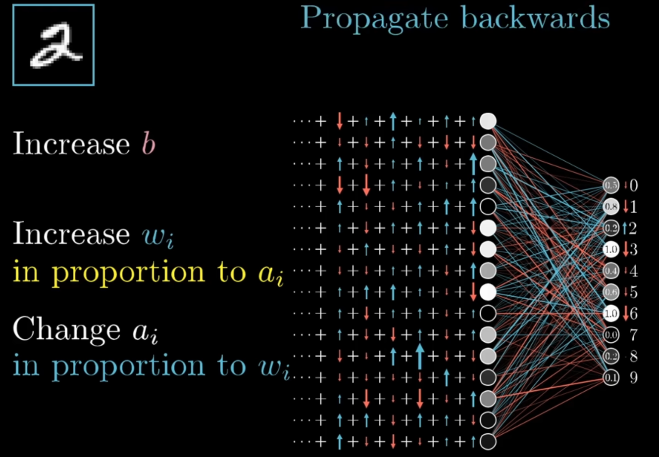

- The figure shows how the desired change in the final output is translated into parameter updates in the last layer and then propagated backward to determine how the previous layer should change. - See details: [[Single Neuron Computation]] ### Example - The output is 0.5, but the correct value should be 0. - This means the neuron's output is too high and should be **nudged** downward. - There are three things to consider: - Adjust the bias - If the neuron is too active, decrease its bias. - Adjust the weights - If a previous activation contributed strongly to this high output, decrease the corresponding weight. - Check the previous activations - If a neuron in the previous layer contributed strongly to this error, propagate the signal backward so the **previous** layer can adjust its own weights and bias. - Activations are not directly updated as parameters; they are intermediate values used to propagate the error backward.

Also, if we trained the network using only images of the digit 2, the learned weights and biases would be heavily biased toward predicting 2.

In that case, the network might output something close to 2 for almost every input.

To learn meaningful weights and biases, the network must be trained on many different examples from different classes. During training, we randomly sample examples or mini-batches from the dataset to estimate the gradient and update the parameters. This is the basic idea behind stochastic gradient descent.

Stochastic Gradient Descent (SGD):

• Since using the entire training set for every parameter update is computationally expensive, we instead use small mini-batches of data
• (for example, 100 training examples) to approximate the gradient. This makes training much faster, although the path down the cost surface becomes noisier and less precise.

Formula

Name	Formula	Meaning	Purpose
Output layer error	${\delta }^L={\nabla }_{a}C\odot {\sigma }^{\prime }(z^L)$	output error signal = cost sensitivity × activation slope	Compute the error signal for the output layer.
Hidden layer error	${\delta }^l=((W^{l+1}{)}^T{\delta }^{l+1})\odot {\sigma }^{\prime }(z^l)$	backpropagated next-layer error × local activation slope	Compute the error signal for a hidden layer.
Bias gradient	$\frac{\partial C}{\partial b_j^l}={\delta }_j^l$	bias gradient = neuron error signal	The gradient of the bias equals the neuron’s error signal.
Weight gradient	$\frac{\partial C}{\partial w_{jk}^l}=a_k^{l-1}{\delta }_j^l$	weight gradient = input activation × output neuron error	The gradient of a weight equals input activation times output error signal.

• See Details: Symbol ∇ nabla

Backpropagation Formula Flow

output error → hidden error → bias gradient → weight gradient → update parameters

• First, compute the output error signal.
• Then, use it to compute the hidden layer error signal by passing the error backward through the weights.
• Once a layer’s error signal is known:
  • its bias gradient is that error signal
  • its weight gradient is previous activation × current error signal
• Finally, update the weights and biases.

Formula: Output layer error

• output: Error signal
• Purpose: to determine how much each neuron in the output layer contributes to the overall error.
• Meaning: the error at the output layer equals the cost sensitivity times the activation slope.

At the output layer:
${\delta }^L={\nabla }_{a}C\odot {\sigma }^{\prime }(z^L)$

• Cost sensitivity measures how much the cost cares about the output, while activation slope measures how easily the neuron output changes with respect to its input.
• cost sensitivity = ${\nabla }_{a}C$
• activation slope = ${\sigma }^{\prime }(z^L)$
• Symbol:
  • ${\delta }^L$ : delta
    • error / sensitivity of the output layer (the error signal for each neuron in layer $L$)
  • ${\nabla }_{a}C$ : nabla
    • gradient of the cost function with respect to the output activations $a$
    • ${\sigma }^{\prime }(z^L)$ : sigma
    • derivative of the activation function evaluated at $z^L$
  • $\odot$ : element-wise multiplication (Hadamard product)
    • $z^L$ : weighted input of the output layer, computed as $z^L=W^L{a}^{L-1}+b^L$
    • $C$ : cost (loss) function that measures how far the prediction is from the target

Hadamard product

$\odot$ : element-wise multiplication (Hadamard product)

Example:

• Meaning: multiply corresponding elements position by position.
• e.g. $\left[\begin{array}{c}1\\ 2\\ 3\end{array}\right]\odot \left[\begin{array}{c}4\\ 5\\ 6\end{array}\right]=\left[\begin{array}{c}4\\ 10\\ 18\end{array}\right]$

1. What is Cost Sensitivity?

Cost sensitivity means:

If a changes a little, how much does cost change?
how much the cost changes if the output activation changes a little.

• Mathematically: $\frac{\partial C}{\partial a}$

• For neuron $j$ in the output layer: $\frac{\partial C}{\partial a_j^L}$

• Meaning: if the output $a_j^L$ changes slightly, how much will the cost change?

Example: Quadratic Cost

• If the cost function is $C=\frac{1}{2}(a-y{)}^2$

  • Make the partial derivative easier and cleaner by adding 1/2.

• Then $\frac{\partial C}{\partial a}=a-y$

• So in this case: cost sensitivity = prediction − target

• Example 1

  • If:
    • prediction $a=0.8$
    • target $y=1$
  • Then
    • $\frac{\partial C}{\partial a}=0.8-1=-0.2$

• Example 2

  • If:
    • prediction $a = 0.8
    • target $y=0$
  • Then
    • $\frac{\partial C}{\partial a}=0.8-0=0.8$

Interpretation: If prediction and target differ a lot, the sensitivity will be large.

2. What is Activation Slope?

if z changes a little, how much does a change?

• $z=Wa+b$
• $a^{l-1}\to z^l\to a^l$
• activation function = $\sigma$ (sigma)
• $a^l=\sigma (z^l)$

Activation slope means: the derivative of the activation function.

• If
  • $a=\sigma (z)$
• then
  • ${\sigma }^{\prime }(z)$
• represents how much the output activation changes if the input $z$ changes.

If the activation function is Sigmoid

• Sigmoid:

  • $\sigma (z)=\frac{1}{1+e^{-z}}$

• Derivative:

  • ${\sigma }^{\prime }(z)=\sigma (z)(1-\sigma (z))$

• Since $a=\sigma (z)$, we often write

  • ${\sigma }^{\prime }(z)=a(1-a)$

• Example

  • If a neuron’s output activation is $a=0.8$
  • Then ${\sigma }^{\prime }(z)=a(1-a)=0.8(1-0.8)=0.16$
  • So the activation slope = 0.16.

If the activation function is ReLU

• ReLU: $\mathrm{ReLU}(z)=\max (0,z)$

• Derivative: ${\mathrm{ReLU}}^{\prime }(z)=\{\begin{array}{ll}1,& z>0\\ 0,& z<0\end{array}$

• So:

  • if $z>0$, activation slope = 1
  • if $z<0$, activation slope = 0

3. Combining the Two

For a single neuron at the output layer:
$\delta =\frac{\partial C}{\partial a}\cdot {\sigma }^{\prime }(z)$
This means:

neuron error = cost sensitivity × activation slope

Example: Sigmoid + Quadratic Cost

• Assume:
  • target $y=1$
  • output $a=0.8$
• Step 1 — Cost Sensitivity
  • $\frac{\partial C}{\partial a}=a-y=0.8-1=-0.2$
• Step 2 — Activation Slope
  • ${\sigma }^{\prime }(z)=a(1-a)=0.8(1-0.8)=0.16$
• Step 3 — Multiply
  • $\delta =(-0.2)\times 0.16=-0.032$
    This value is the error signal for that output neuron.