DL4 Backpropagation calculus

• Youtube: Backpropagation calculus | Deep Learning Chapter 4

Key Takeaway

• $\partial C/\partial w$ = how wrong the output is × how responsive the neuron is × how active the input was
• These three factors come from the chain rule applied along the path $w\to z\to a\to C$
• When one neuron feeds into many next-layer neurons, those contributions sum
• This chain-rule structure is the mathematical core of backpropagation

This chapter answers:

Why do the formulas in backpropagation look the way they do?
What does the chain rule actually mean inside a neural network?

Introduce

This chapter takes the intuition from DL3 Backpropagation (intuitively) and rewrites it in the language of calculus.

• Chapter 3 focuses on intuition:
  • The output layer is wrong, and responsibility is passed backward layer by layer.
• Chapter 4 focuses on formulas:
  • How to compute the partial derivatives of the cost with respect to each weight and bias.
• Core message of the video:
  • In machine learning, the chain rule is best understood as a way of tracking how influence propagates through a computation.

---

Main Idea of the Video

The chapter starts with an extremely simple network:

• one neuron per layer
• three weights and three biases in total
• attention focused only on the connection between the last two neurons

Why start with such a simple setup?

• Because the essence of backpropagation is not complicated.
• What makes it look complicated is:
  • many symbols
  • many indices
  • many dependencies across layers
• Once the chain rule is clear along a single path, the multi-neuron case is mostly the same idea with more bookkeeping.

---

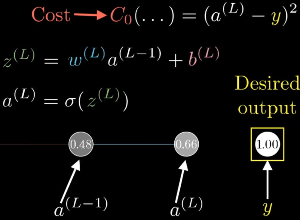
Single-Neuron Version: Fix the Notation First

We look only at one neuron in the final layer. Use the following notation:

• $a^L$
  • the activation of layer $L$, the final output
• $a^{L-1}$
  • the activation of the previous layer
• $w^L$
  • the weight connecting $a^{L-1}$ to $a^L$
• $b^L$
  • the bias of the final neuron
• $z^L$
  • the weighted input, or pre-activation
• $y$
  • the target value for this training example
• $C_0$
  • the cost for this single training example

Forward computation:

$$z^L=w^L{a}^{L-1}+b^L$$ $$a^L=\sigma (z^L)$$

For a single training example, using squared error:

$$C_0=(a^L-y{)}^2$$

The key dependency chain is:

$$w^L,b^L,a^{L-1}\to z^L\to a^L\to C_0$$

So the weight does not affect the cost directly. It affects the cost only through intermediate variables.

---

What the Chain Rule Means Here

What we really want is:

$$\frac{\partial C_0}{\partial w^L}$$

This means:

• if we nudge $w^L$ a little
• how much does the cost change?

The video breaks this into three steps:

1. a small change in $w^L$ changes $z^L$
2. a small change in $z^L$ changes $a^L$
3. a small change in $a^L$ changes $C_0$

So:

$$\frac{\partial C_0}{\partial w^L}=\frac{\partial C_0}{\partial a^L}\cdot \frac{\partial a^L}{\partial z^L}\cdot \frac{\partial z^L}{\partial w^L}$$

This is the central chain-rule view behind backpropagation:

Total sensitivity = product of local sensitivities

Instead of treating it as a memorized formula, it is better to see it as:

• influence traced backward through the graph
• responsibility propagated backward through the computation

---

03:55 The Three Local Derivatives

1. Derivative of Cost with Respect to Output Activation

• From $C_0=(a^L-y{)}^2$

• we get $\frac{\partial C_0}{\partial a^L}=2(a^L-y)$

• Meaning:

  • the farther the output is from the target, the more sensitive the cost is to the output

So this term tells you: how wrong the current prediction is

• If $a^L$ is already close to $y$, this term is small.

2. Derivative of Activation with Respect to Weighted Input

• Since $a^L=\sigma (z^L)$

• we have $\frac{\partial a^L}{\partial z^L}={\sigma }^{\prime }(z^L)$

Meaning:

• this measures how sensitive the neuron is at its current input value
• even if the output error is large, the signal can be damped if the activation function is locally flat

If the activation function is sigmoid: ${\sigma }^{\prime }(z)=\sigma (z)(1-\sigma (z))$

If the activation function is ReLU: ${\mathrm{ReLU}}^{\prime }(z)=\{\begin{array}{ll}1,& z>0\\ 0,& z<0\end{array}$

3. Derivative of Weighted Input with Respect to Weight

Since

$$z^L=w^L{a}^{L-1}+b^L$$

we get

$$\frac{\partial z^L}{\partial w^L}=a^{L-1}$$

This term carries an important intuition:

The stronger the previous neuron fires, the more changing this weight matters.

This is where the idea

• neurons that fire together wire together

starts to show up mathematically.
If the previous neuron is barely active, adjusting this weight will not change much.

---

04:40 Put Them Together: Gradient of the Final-Layer Weight

w → z → a → C

Multiply the three local derivatives:

= \frac{\partial C_0}{\partial a^L} \cdot \frac{\partial a^L}{\partial z^L} \cdot \frac{\partial z^L}{\partial w^L} =2(a^L-y)\sigma'(z^L)a^{L-1}$$ This is the gradient of the final-layer weight for one training example. You can read it as three factors: - $2(a^L-y)$ - how wrong the output is - $\sigma'(z^L)$ - how easy the neuron is to push at this point - $a^{L-1}$ - how active the input to this connection is Together, these determine whether the weight should change and by how much. --- # 05:10 From One Training Example to the Whole Dataset So far we computed the cost for a single example, $C_0$. But during training, we optimize the average cost across the dataset:

C = \frac{1}{n}\sum_{x} C_x

$$Sothefullgradientistheaverageofthesingle-examplegradients:$$

\frac{\partial C}{\partial w^L}

\frac{1}{n}\sum_x
\frac{\partial C_x}{\partial w^L}

This explains the division of labor: - backpropagation computes gradients - gradient descent uses those gradients to update parameters In mini-batch SGD, we average over a small batch instead of the whole dataset. --- # 05:45 The Bias Gradient Is Almost the Same For the bias, we only replace the last factor:

\frac{\partial C_0}{\partial b^L}

\frac{\partial C_0}{\partial a^L}
\cdot
\frac{\partial a^L}{\partial z^L}
\cdot
\frac{\partial z^L}{\partial b^L}

$$And$$

\frac{\partial z^L}{\partial b^L}=1

$$So:$$

\frac{\partial C_0}{\partial b^L}

2(a^L-y)\sigma’(z^L)

So the bias gradient is almost the same as the weight gradient, except it does not include the input activation $a^{L-1}$. That makes sense: - a weight scales one particular incoming signal - a bias shifts the neuron as a whole --- # 06:05 What Is Actually Being Propagated Backward? This is where the video explains the name **backpropagation**. Even though we do not directly update $a^{L-1}$, we still want:

\frac{\partial C_0}{\partial a^{L-1}}

$$Why?-becauseittellsushowsensitivethefinalcostistothepreviouslayer-andthatletsuskeepmovingbackwardtocomputeearliergradientsUsingthechainruleagain:$$

\frac{\partial C_0}{\partial a^{L-1}}

\frac{\partial C_0}{\partial a^L}
\cdot
\frac{\partial a^L}{\partial z^L}
\cdot
\frac{\partial z^L}{\partial a^{L-1}}

$$And$$

\frac{\partial z^L}{\partial a^{L-1}} = w

$$So:$$

\frac{\partial C_0}{\partial a^{L-1}}

2(a^L-y)\sigma’(z^L)w

This is the mathematical form of passing responsibility backward: - take the current error signal - multiply by the relevant weight - send it back to the previous layer Then the same logic repeats layer by layer. --- # 06:45 Extend to Multiple Neurons Per Layer A real network has many neurons per layer, but the core idea does not change much. The main difference is: > There is no fundamentally new idea here, only more indices. Now use this notation: ![[pic_c4p2.png]] - $a_j^L$ - activation of neuron $j$ in layer $L$ - $a_k^{L-1}$ - activation of neuron $k$ in layer $L-1$ - $w_{jk}^L$ - weight from neuron $k$ in layer $L-1$ to neuron $j$ in layer $L$ - $b_j^L$ - bias of neuron $j$ in layer $L$ - $z_j^L$ - pre-activation of neuron $j$ in layer $L$ - $y_j$ - target value for output neuron $j$ Forward equations:

z_j^L = \sum_k w_{jk}^L a_k^{L-1} + b_j

a_j^L = \sigma(z_j^L)

$$Single-examplecost:$$

C_0 = \sum_j (a_j^L - y_j)

This matches the multi-output setup from Chapters 2 and 3. --- # 07:55 Gradient of One Specific Weight in the Multi-Neuron Case If we focus on one particular weight $w_{jk}^L$, the chain-rule structure is almost identical:

\frac{\partial C_0}{\partial w_{jk}^L}

\frac{\partial C_0}{\partial a_j^L}
\cdot
\frac{\partial a_j^L}{\partial z_j^L}
\cdot
\frac{\partial z_j^L}{\partial w_{jk}^L}

$$Eachtermis:$$

\frac{\partial C_0}{\partial a_j^L}=2(a_j^L-y_j)

\frac{\partial a_j^L}{\partial z_j^L}=\sigma’(z_j^L)

\frac{\partial z_j^L}{\partial w_{jk}^L}=a_k^{L-1}

$$So:$$

\frac{\partial C_0}{\partial w_{jk}^L}

2(a_j^L-y_j)\sigma’(z_j^L)a_k^{L-1}

$$Thisisexactlythesamestructureasbefore,nowwithindices.Forthebias:$$

\frac{\partial C_0}{\partial b_j^L}

2(a_j^L-y_j)\sigma’(z_j^L)

--- # 08:30 Why Does a Sum Appear When Propagating to the Previous Layer? This is the most **important** extension in the video. ![[pic_c4p3.png]] The screenshot is showing the weight-gradient formula, together with what should be plugged into the boxed term:

\frac{\partial C}{\partial w_{jk}^{(l)}}

a_k^{(l-1)} \sigma’(z_j^{(l)}) \frac{\partial C}{\partial a_j^{(l)}}

The yellow box is explaining how to compute $$\frac{\partial C}{\partial a_j^{(l)}}$$ depending on where that neuron is: - If it is in a **hidden** layer, that quantity comes from summing all contributions from the next layer: (k `layer`, j `layer + 1`)

\frac{\partial C}{\partial a_k^{(l)}}

\sum_{j=0}^{n_{l+1}-1}
w_{jk}^{(l+1)} \sigma’(z_j^{(l+1)}) \frac{\partial C}{\partial a_j^{(l+1)}}

$$-Ifitisalreadyinthe\ast \ast output\ast \ast layer,thestartingpointis:$$

\frac{\partial C}{\partial a_j^{(L)}} = 2(a_j^{(L)} - y_j)

In the one-neuron case, $a^{L-1}$ influences the cost through only one path. But in the multi-neuron case, a previous-layer activation $a_k^{L-1}$ can affect many neurons in the next layer: - it affects $a_0^L$ - it affects $a_1^L$ - and possibly many more $a_j^L$ So its total influence on the cost is no longer one chain. It is the sum of many paths:

\frac{\partial C_0}{\partial a_k^{L-1}}

\sum_j
\frac{\partial C_0}{\partial z_j^L}
\cdot
\frac{\partial z_j^L}{\partial a_k^{L-1}}

Meaning: - We are asking how changing one activation $a_k^{L-1}$ would change the final cost. - That activation does not affect just one next-layer neuron. It affects every neuron $a_j^L$ connected to it. - Each connection creates one path from $a_k^{L-1}$ to the cost. - So we compute the contribution from each path and then add them together. This is why the formula is a sum:

\frac{\partial C_0}{\partial a_k^{L-1}}

\text{(path through neuron 0)}
+
\text{(path through neuron 1)}
+
\cdots

$$‘k->j‘Where$$

\frac{\partial C_0}{\partial z_j^L}

\frac{\partial C_0}{\partial a_j^L}
\cdot
\frac{\partial a_j^L}{\partial z_j^L}

2(a_j^L-y_j)\sigma’(z_j^L)

$$and$$

\frac{\partial z_j^L}{\partial a_k^{L-1}} = w_{jk}

$$Therefore:$$

\frac{\partial C_0}{\partial a_k^{L-1}}

\sum_j 2(a_j^L-y_j)\sigma’(z_j^L)w_{jk}

That summation appears because: > One neuron in the previous layer influences the cost through multiple outgoing paths. This is the key new feature when moving from a single chain to a real layer. --- # 09:00 Connect This to Standard Backpropagation Notation The video does not emphasize the $\delta$ notation, but adding it makes the result easier to connect to standard textbooks. Define:

\delta_j^L := \frac{\partial C_0}{\partial z_j^L}

$$Thenfortheoutputlayer:$$

\delta_j^L = 2(a_j^L-y_j)\sigma’(z_j^L)

$$So:$$

\frac{\partial C_0}{\partial b_j^L} = \delta_j

\frac{\partial C_0}{\partial w_{jk}^L} = a_k^{L-1}\delta_j

$$Andwhenpropagatingbackward:$$

\frac{\partial C_0}{\partial a_k^{L-1}}

\sum_j w_{jk}^L \delta_j

$$Ifwethenmultiplybythederivativeofthepreviouslaye{r}^{\prime }sactivationfunction,wegetthehidden-layererrorsignal:$$

\delta_k^{L-1}

\left(\sum_j w_{jk}^L \delta_j^L\right)\sigma’(z_k^{L-1})

This matches the standard formulas from [[DL3 Backpropagation (intuitively)]]. --- # Matrix Form In matrix form, the same ideas become more compact. Output-layer error:

\delta^L = \nabla_{a^L} C_0 \odot \sigma’(z^L)

$$Ifthecostissquarederror:$$

\nabla_{a^L} C_0 = 2(a^L-y)

$$So:$$

\delta^L = 2(a^L-y)\odot \sigma’(z^L)

$$Parametergradients:$$

\frac{\partial C_0}{\partial b^L} = \delta

\frac{\partial C_0}{\partial W^L} = \delta^L (a^{L-1})

$$Hidden-layererrorpropagation:$$

\delta^{l} = ((W^{l+1})^T\delta^{l+1}) \odot \sigma’(z^{l})

These are the standard backpropagation equations used in most neural-network texts. --- # Study Notes ## 1. See Dependencies Before Derivatives Do not start by memorizing formulas. Start by asking: - what does this variable affect? - what intermediate nodes lie between it and the cost? - is there one path or many paths? Once the dependency structure is clear, the chain rule becomes natural. ## 2. A Weight Gradient Has Three Ingredients

\frac{\partial C_0}{\partial w_{jk}^L}

\text{output error}
\times
\text{activation slope}
\times
\text{input activation}

That is: - how wrong the output is - how responsive the neuron currently is - how active this input channel is ## 3. Backprop Does Not Update Activations During backpropagation, we compute quantities like:

\frac{\partial C_0}{\partial a_k^{l}}

But activations are not parameters, so they are not directly updated. They serve as intermediate sensitivities that help compute the gradients of earlier weights and biases. ## 4. The Sum in the Multi-Neuron Case Is Easy to Miss In the single-neuron case, there is only one path, so no sum appears. In the multi-neuron case, one neuron usually influences multiple neurons in the next layer, so all path contributions must be added together. --- # One-Page Summary - Backpropagation calculus treats a neural network as a composition of many small functions. - A parameter affects the cost through a path such as - parameter $\rightarrow z \rightarrow a \rightarrow C$ - For a single output neuron:

\frac{\partial C_0}{\partial w^L}

2(a^L-y)\sigma’(z^L)a^{L-1}

$$-Forthemulti-outputcase:$$

\frac{\partial C_0}{\partial w_{jk}^L}

2(a_j^L-y_j)\sigma’(z_j^L)a_k^{L-1}

$$-Forthebias:$$

\frac{\partial C_0}{\partial b_j^L}

2(a_j^L-y_j)\sigma’(z_j^L)

$$-Whenpropagatingbacktothepreviouslayer,contributionsfromalloutgoingpathsmustbesummed:$$

\frac{\partial C_0}{\partial a_k^{L-1}}

\sum_j 2(a_j^L-y_j)\sigma’(z_j^L)w_{jk}

- This logic of multiplying local derivatives and summing over paths is the mathematical core of backpropagation. --- # Review Questions 1. Why does $\frac{\partial C_0}{\partial w^L}$ break into a product of three local derivatives? 2. What role does $\sigma'(z^L)$ play in the formula? 3. Why is the bias gradient almost the same as the weight gradient, except for the factor $a^{L-1}$? 4. Why must $\frac{\partial C_0}{\partial a_k^{L-1}}$ include a summation in the multi-neuron case? 5. If squared error were replaced with cross-entropy, which part of the formulas would change? --- # Connection - Previous chapter: [[DL3 Backpropagation (intuitively)]] - Good next things to reinforce: - output-layer error $\delta^L$ - hidden-layer error $\delta^l$ - matrix-form backpropagation - If the chain rule still feels abstract, revisit the single-neuron example until the dependency structure feels obvious